Cascade-Correlation architecture

February 01, 2019

Stefano Martina

---

Cascade-Correlation is an architecture developed in 1990 by Scott E. Fahlman and Christian Lebiere [Fahlman1990] . It introduces two concepts:

• a cascade architecture where hidden units are appended incrementally to the network and do not change after they are added;
• a learning algorithm that for each added units attempt to maximise the correlation between it’s output and residual error of preexisting network.

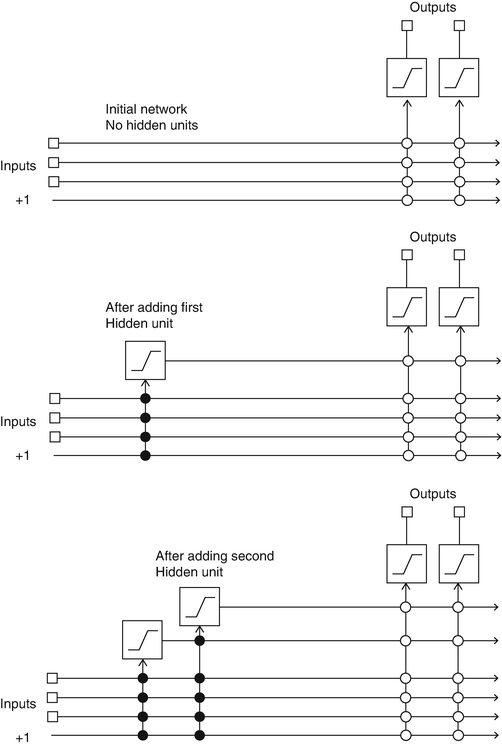
Fig 1 resumes the learning algorithm. Initially the network has only inputs signals and output units, both defined by the problem. Output unit are trained with backpropagation¹ until no significant error reduction occurs. If the network’s performance are not satisfying, a new unit is attached and trained in a twofold process.

1. A candidate unit is created with trainable input connections attached to network input and existing hidden units. Its output is not connected to the network, and its trained maximizing the correlation with its output and the network residual error.
2. The candidate unit is installed in the network: its input are frozen and the output is connected to network’s output units. After the process restart training network’s output units with backpropagation.

The correlation between a candidate unit and the network’s residual error is expressed with:

$$\begin{equation*} S = \sum_o\left|\sum_p(V_p - \overline V)(E_{p,o} - \overline{E}_o)\right|, \end{equation*}$$

where $o$ are network output units, $p$ training samples, $V_p$ is candidate unit’s output for sample $p$, $E_{p,o}$ residual error of output unit $o$ for sample $p$ and $\overline{V}$, $\overline{E}_o$ are the corresponding averaged over all samples.

In order to maximize $S$, gradient ascend with backpropagation on the single unit is performed until it stop improving. The differentiation of $S$ for weight $i$ is:

$$\begin{equation*} \frac{\partial S}{\partial w_i} = \sum_{p,o}\sigma_o(E_{p,o}-\overline{E}_o)f_p'I_{i,p}, \end{equation*}$$

where $\sigma_o$ is the sign of correlation between unit and network outputs, $f_p’$ is the derivative of unit’s activation function respect its inputs sum, and $I_{i,p}$ is the input from unit $i$ and sample $p$.

To improve the method is possible to parallelly train a pool of candidate units with different set of random weight. The candidate with better correlation score is thus selected.

The architecture is quite old, but it has some advantages:

• the learning algorithm guesses network’s correct size;
• learning is fast because only one layer per time is trained;
• a deep network is built without the negative effect (i.e. vanishing gradient);
• cascade-correlation is useful for incremental learning, a feature detector is never cannibalized (i.e. catastrophic forgetting).

---

References

---

Footnotes